Introduction to Neural Networks
What Is a Neural Network?
A neural network is inspired by the information processing of neurons. The most common networks learn by example. These networks are taught how to produce correct outputs by training them against large datasets of input-output pairs. It is nearly impossible to reverse engineer exactly how a particular network works. This may not be the case in the future as work is being done to glean insight into these powerful models.
How does one make a neural network? It begins by deciding the architecture. All common architectures include one or more layers, a number of neurons in each layer, what types of neurons are used, and the types of connections between neurons in adjacent layers. The architecture of a network is like the connectome of a brain.
An architecture needs a dataset to train on. A dataset will usually contain desired input and output pairs that the network must learn to correlate. There are cases where pairs are not necessary, the distribution of the data used to learn instead.
A network is trained with an input-output pair by passing the input through it and comparing the result to the output of the pair. The network will produce noise in the beginning. The error between the result and desired output is calculated. For every adjustable parameter in the network, it is calculated. This is repeated many times until the error is reduced to a minimal amount.
Example Networks
Here are some example networks to give an idea of the kinds of problems neural networks can solve.
A Neural Algorithm of Artistic Style
Progressive Growing of GANs for Improved Quality, Stability, and Variation
Unsupervised Image-to-Image Translation Networks
Phase-Functioned Neural Networks for Character Control
Structure of a Neural Network
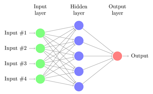
A neural network is built out of layers of interconnected neurons. The first layer is called the input layer and receives samples directly from dataset as input, the middle layers are called the hidden layers and take the previous layer’s output as input. The last layer is called the output layer and outputs the final result of the network.
The fact that each layer passes its output to the next makes this a description of a feedforward neural network. Since each layer transforms data from the previous layer, the deeper the layer the more abstract the information at that layer becomes. This is powerful because it allows the network to learn high level features, such as if someone is smiling or frowning in a photograph.
Every network also needs a loss function, which measures the difference between an output and the expected output, and an optimizer that uses the loss to determine how to shift the network’s weights.
Layer Connections
Layers in a neural network are typically fully connected; each neuron in a layer gets its inputs from every neuron in the previous layer. Sometimes these connections are altered such as in the case of residual networks, where the inputs can be fed to multiple layers.
Dropout
Dropout is another method of connecting layers. Dropout will randomly disconnect a given percentage of connections between two layers during training. This may sound like it would break the network, but it actually makes it more robust. The network learns how to arrive at the correct answer even with missing data. Once the network is fully trained and is being applied, dropout is no longer enabled and all the connections are active. The connections are scaled to account for the extra active connections.
Dropout reduces the problem of overfitting, which is when the network is plagiarizing the training data instead of generalizing it. This is like learning by memorization as opposed to learning by understanding.
Loss Function
A loss function is a measure of how dissimilar two things are. A loss of zero should mean the two things being measured are identical. An example loss function would be the distance between two points in space: If the distance is 0 the points are identical, with increasing distances indicating that the points are less and less similar.
A common loss function is the squared error. You take the difference between two numbers and square it. This has the benefit of keeping the loss positive, and penalizing larger differences.
Optimizer
An optimizer is a process that uses the loss function and dataset to determine how to change the parameters (weights) of the network.
Stochastic gradient descent (SGD) is the optimization process of running a sample input from the dataset through the network, then using the derivative of the loss with respect to the parameters of the network to nudge those parameters in a direction that lowers that loss. This derivative is called the gradient.
Mini-batch gradient descent is the same process except the gradients from a batch of random samples from the dataset are averaged. This helps ensure the gradient is pointing in a direction that optimizes in a general way for many sample inputs and not just individual inputs.
There are variants of gradient descent such as ones that involve momentum and adaptive learning rates which you can read more about here.
Anatomy of a Neuron
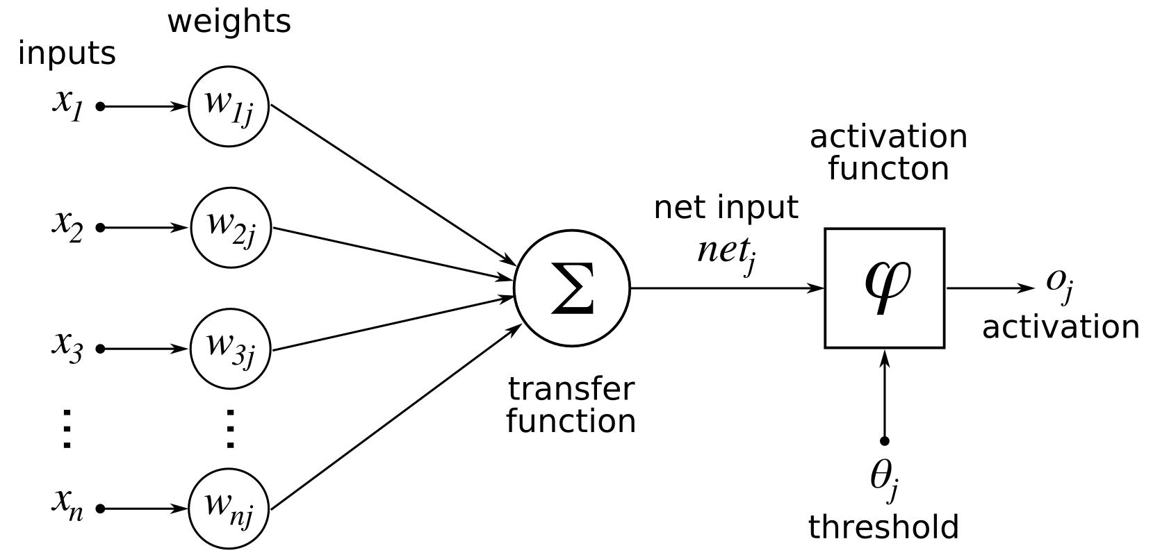
Artificial neurons act in a similar manner to biological neurons by propagating signals between each other. A typical artificial neuron consists of inputs, weights, a bias, and an activation function.
Inputs
The input layer’s inputs come from the dataset. Subsequent layers are fed the sum of weighted activations plus bias (\(\sum wa+b\)) from the previous layer.
Weights
Each weight (\(w\)) scales the respective activation from the previous layer. They are parameters of the network that are learned.
Bias
The bias (\(b\)) is a parameter simply added to the sum of weighted activations (\(\sum wa\)).
It turns out the bias is conceptually the same as a weight where the corresponding activation is always \(1\). We can exploit this to prevent the model from becoming more complex than it needs to be. To simulate the bias, an extra input is fed into every neuron. This input is set to a constant value of \(1\).
Activation Function
The activation function is a function that defines the output of a neuron. Activation functions are typically chosen to bound the output between a range of values. Popular activation functions are the sigmoid, tanh, RELU, ELU, and softmax functions. The tanh function is nice as it balances the output between \(-1\) and \(1\).

This is like a continuous form of a binary choice: A large negative value becomes \(-1\), and a large positive value becomes \(1\), with smaller numbers somewhere in-between.
The non-linearity of this function is what makes the whole network non-linear. This non-linearity is what allows neural networks to approximate any function.
Vanishing Gradient Problem
The vanishing gradient problem is an issue where a neural network’s training slows down the farther back in the network the gradient is propagated. In the case of the tanh function, its derivative will always be between \(0\) and \(1\). This means that for every layer the gradient is propagated through, the gradient is multiplied by some value between \(0\) and \(1\). Do this enough times and the gradient becomes smaller and smaller until it “vanishes”. The effect this has is that the farther from the end of the network a layer is, the less it will be updated by the gradient.
Attempts at a solution to the vanishing gradient problem include the residual networks mentioned previously, and recurrent LSTM networks.
Training a Neural Network
Backpropagation
Backpropagation is the meat of a neural network’s training algorithm. It relies on using the gradient, the derivative of the loss with respect to the parameters of the network. With this gradient one can update the parameters of the network to reduce the loss, which will make the network perform better.
Before one can use backpropagation, the gradient must be found. An input from the dataset is fed into the network. Then the output of the network is compared to the corresponding expected output using a loss function like the squared error.
Once the loss is computed we can find the derivative of the loss with respect to the weights of the last layer of neurons. Using the notation from earlier, this is \(\frac{\partial C}{\partial w^{L}}\) where \(C\) is the loss of the function, and L is the total number of the layers in the network.
This is where backpropagation begins. Remember the chain rule from calculus? A brief reminder: If you multiply two derivatives such that terms cancel out, you get another valid derivative. For example, \(\frac{\ \partial b}{\partial a} \cdot \frac{\partial c}{\partial b} = \frac{\partial c}{\partial a}\). This can be applied to the neural network too. If you can find \(\frac{\partial w^{L}}{\partial w^{L-1}}\), you can use the chain rule to easily also find \(\frac{\partial C}{\partial w^{L-1}} = \frac{\partial C}{\partial w^{L}} \cdot \frac{\partial w^{L}}{\partial w^{L-1}}\).
You repeat this process for each layer until it has gone through the whole network. Then you have the gradient for the entire network, which describes how the loss changes for any particular weight. The weights can then be updated by subtracting a small multiple of the gradient from the weights. This small multiple is the gradient multiplied by the learning rate, which is often set to decrease over training time to allow the network to settle into a local optimum.
Conclusion
This covers the basics of what one should know about neural networks. There is much more to learn than this but I hope this explanation has given you an idea of how they work. Let me know in the comments if there is anything in this introduction that could be improved upon.