Visualizing Complex Functions
Complex Numbers
Despite the name, complex numbers are easier to understand than they sound. A complex number is actually made of two numbers, or components, a real component and an imaginary component. Think of a complex number as a point on a 2D plane, instead of the usual real number line.
What is an imaginary number? It is any real number multiplied by \(i\) where \(i = \sqrt{-1}\).
A big reason \(i\) is useful is because with it, all polynomials have a root. They make taking the square root or logarithm of negative numbers possible and more. In fact most functions have a natural extension to the complex domain. They also provide way of defining the multiplication and division of 2D vectors, alongside the usual addition and subtraction.
Imaginary is a poor name for them. Gauss’ lateral number is much better. They exist and are as useful as negative numbers!
Cartesian Coordinates
You add the real and imaginary numbers together to get a complex number. This is a bit unusual for the concept of a number, because now you have two dimensions of information instead of just one. Like how one imagines the real numbers as a point on a number line, one can imagine a complex number as a point on a number plane. The x-axis of the number plane represents the real component, and the y-axis represents the imaginary component. This is a Cartesian coordinate system.
\[z = x + yi\]Polar Coordinates
While the axes directly correspond to each component, it is actually often times easier to think of a complex number as a magnitude (\(r\)) and angle (\(\theta\)) from the origin. This way of representing a point on the plane is called a polar coordinate system. The reason it is easier is because when you multiply two complex numbers, the result’s magnitude is the product of the two original magnitudes, and the result’s angle is the sum of the two original angles. \(i\) has a magnitude of \(1\) and an angle of \(\frac{\pi}{2}\) radians (\(90\) degrees) counterclockwise from the positive x-axis, so multiplying by \(i\) can be thought of as rotating a point on the plane by \(\frac{\pi}{2}\) radians counterclockwise.
\[z = r\mathrm{e}^{\theta i}\]The reason why this equation works is outside the scope of this explanation, but it has to do with Euler’s formula.
Complex Functions
A complex function is a function that acts on complex numbers. The function \(f(z) = z^2\) can be extended to the complex domain to take in a complex number and return a complex number. The variable \(z\) is commonly used to represent a complex number, like how \(x\) is commonly used to represent a real number. Let’s see how squaring a complex number affects its real and imaginary components.
In Cartesian coordinates:
\[\begin{split} z &= x + yi \\ z^2 &= (x+yi)^2 \\ z^2 &= x^2 + 2xyi + (yi)^2 \\ z^2 &= x^2 + 2xyi + y^2i^2 \\ z^2 &= x^2 + 2xyi - y^2 \\ z^2 &= (x^2 - y^2) + (2xy)i \\ \end{split}\]In Polar coordinates:
\[\begin{split} z &= r\mathrm{e}^{\theta i} \\ z^2 &= (r\mathrm{e}^{\theta i})^2 \\ z^2 &= r^2\mathrm{e}^{2\theta i} \\ \end{split}\]See how much easier it is to square in polar coordinates? Not only is it simpler, but the result is easy to interpret. The magnitude is squared, and the angle is doubled.
Graphing Complex Functions
Graphing a complex function is surprisingly difficult. A real function takes one dimension of information and outputs one dimension of information. This adds up to a convenient two dimensions, which is easy to display on a computer screen or paper. Complex functions on the other hand take two dimensions of information and output two dimensions, leaving us with a total of four dimensions to squeeze into our graph. This almost sounds impossible, how on earth could we come up with a way to visualize four dimensions?
One way could be to plot a vector field. A vector field is a plot of a bunch of little arrows. Each arrow represents how the point they are on top of gets transformed by the function. This may work but it isn’t very nice as each arrow requires space to draw, which is space that could have been used to draw smaller arrows.
Luckily we have a trick up our sleeve. We can solve this problem by using the polar coordinates from before. There are still a total for four dimensions to plot, except now one of them is cyclic instead of linear. The hues of color are also cyclic. So let’s map the angle to hues.
We have a way to represent the angle, what about the magnitude? For that we’ll use lightness. The less the magnitude the darker it is, the greater the magnitude the lighter it is. There is a glaring problem with this though. Magnitude can be from zero to infinity, and lightness can go from 0% to 100%. To account for this we can break this magnitude up into groups that are each shaded from dark to light, and double them in size each time. For example, one gradient from dark to light will be from magnitudes 1 to 2. Then the next gradient is from 2 to 4, then 4 to 8, and so on. This is not a perfect solution, but it is a good one because doubling is one of the fastest ways to approach infinity.
Summary
Each pixel to be plotted represents a point on the complex plane (\(z\)). This complex number is fed through a function that transforms it (\(f(z) = w\)). This output is represented in polar coordinates (\(w = r\mathrm{e}^{\theta i}\)). The pixel’s hue is mapped to the new angle (\(\theta\)), and the pixel’s lightness is mapped to the new magnitude (\(r\)).
Visualizations
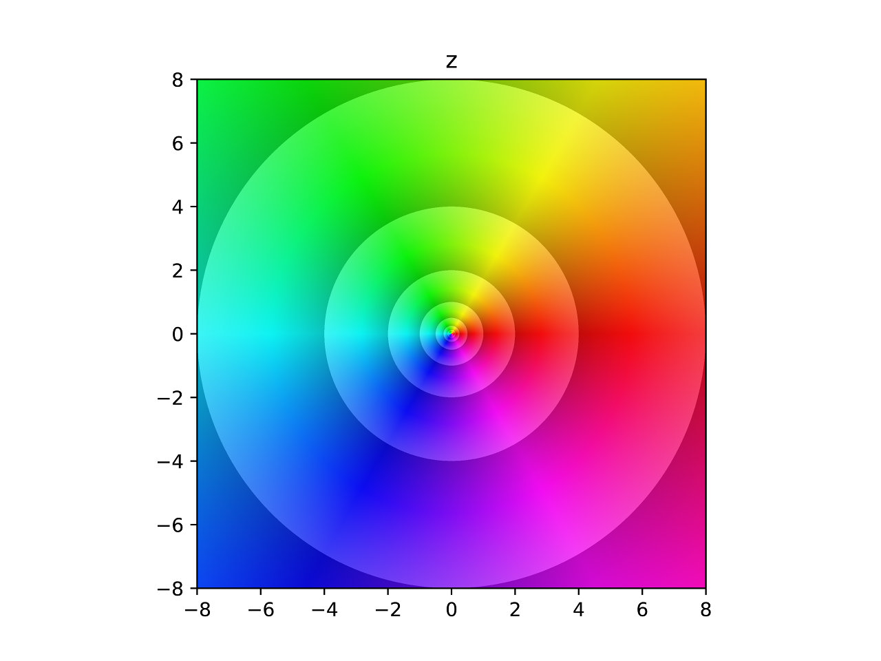
So, what does this look like? Here is the most basic example, the identity function. \(f(z) = z\).
Identity
Square
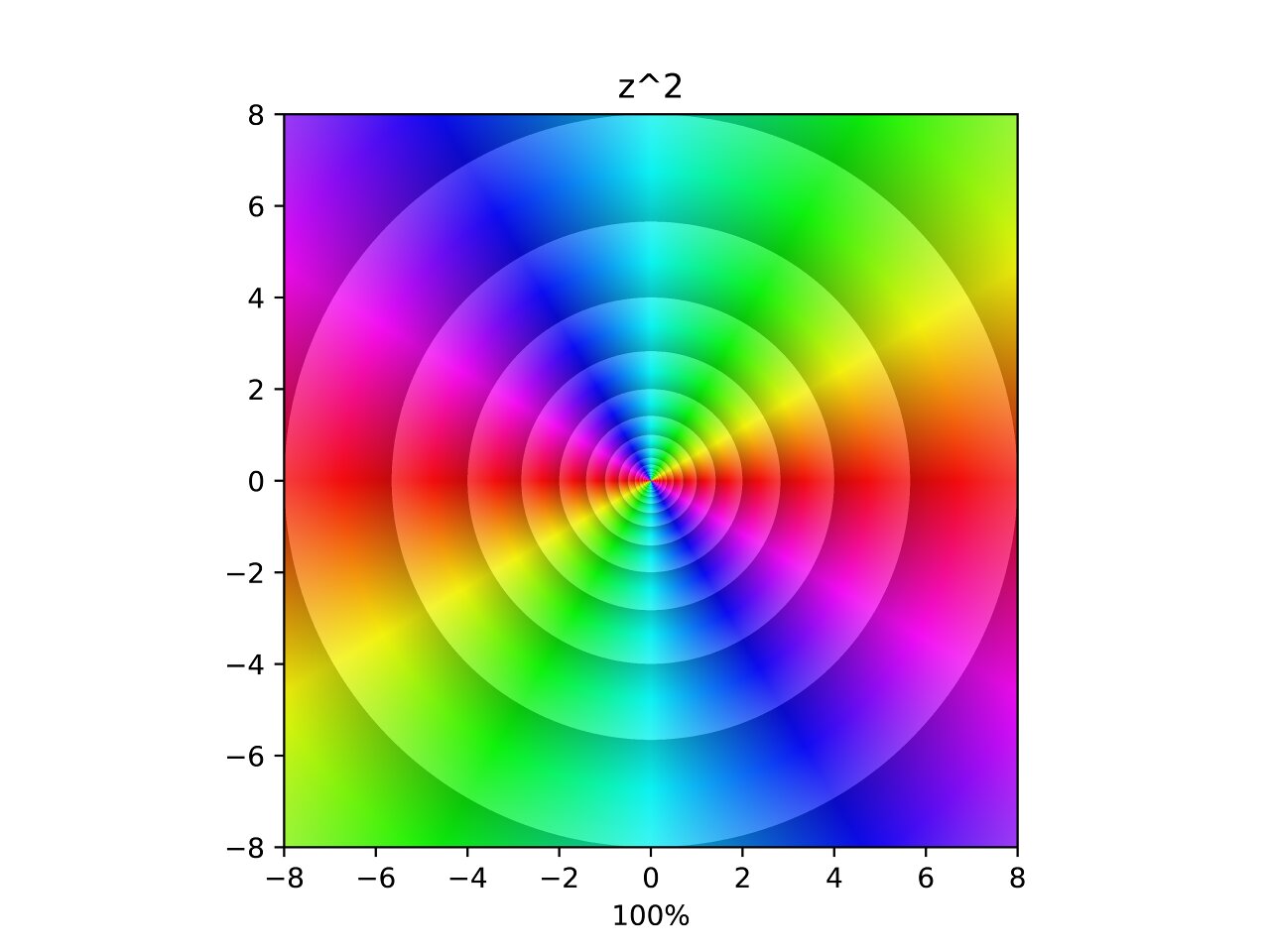
In the image, each hue is repeated twice and the density of the contours has doubled. The video is an interpolation between \(z\) and \(f(z) = z^2\). The points where the contours seem to converge are zeros and poles. Poles are points that diverge to infinity.
From here on I will refer to both zeros and infinities as poles for brevity. Which feels acceptable considering they are both poles on the Riemann sphere.
In this interpolation you can see a pole appear along the negative axis and merge into the original pole. The choice of linear interpolation is rather arbitrary, but it’s curious how the poles move along the animation. Do they trace out interesting curves? Can we come up with a equation for those curves? That’s for another post. For now let’s see the rest!
Cube
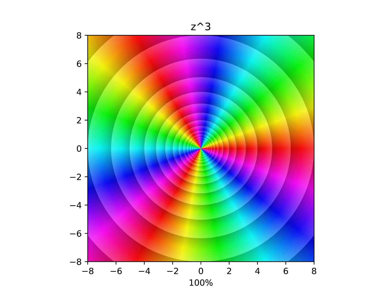
Similarly to the square, this function triples the number of hues around the pole and triples the density of the contours. In the interpolation two additional poles are merged into the original for a total of three poles. Now what happens if we take negative powers?
Inverse
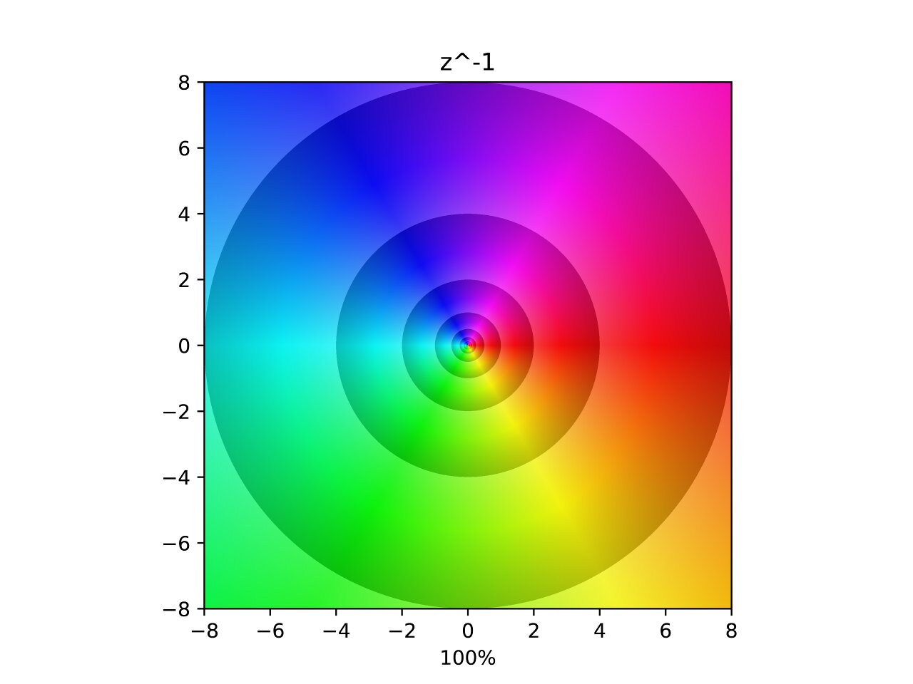
Here you can see what the inverse of the complex plane looks like. The hues are flipped along the horizontal axis and each contour is now halving instead of doubling because the lightness gradient is reversed. In the interpolation one can see two poles being ripped out of the original pole. Which follows the same pattern as the previous two.
Inverse Square
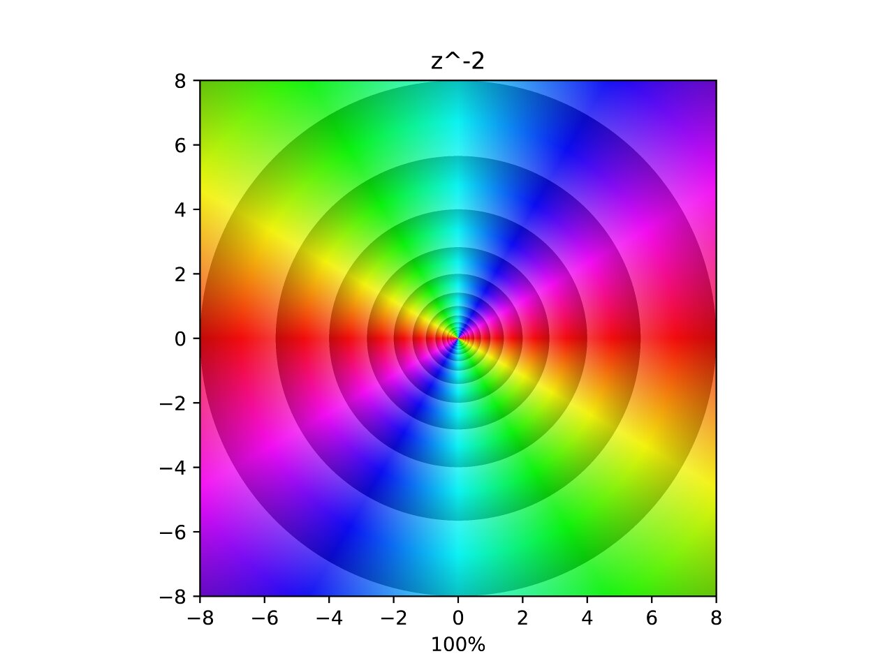
Again following the pattern, three poles are removed from the original. This forms an inverse with two of each hue and double the density of contours
Square Root
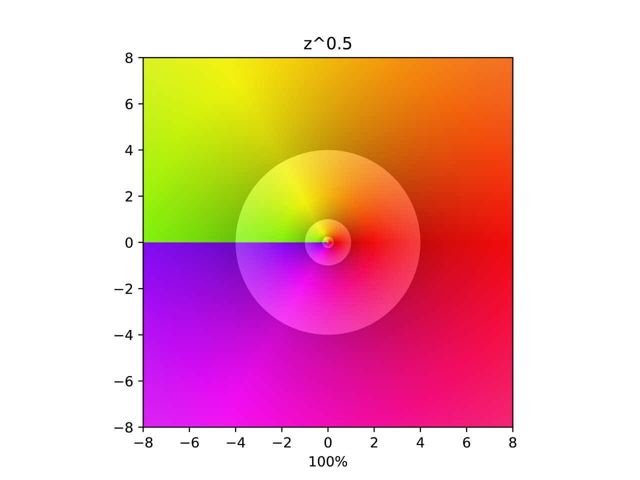
This one is a little strange. Similar to the previous ones except no poles are visibly moving and there is a discontinuity along the negative x-axis called a branch cut. A branch cut means that the function surface gets too complicated to represent in two dimensions, so it is truncated along the negative x-axis for simplicity. I assure you that if you could see four dimensions this function would appear continuous.
Inverse Square Root
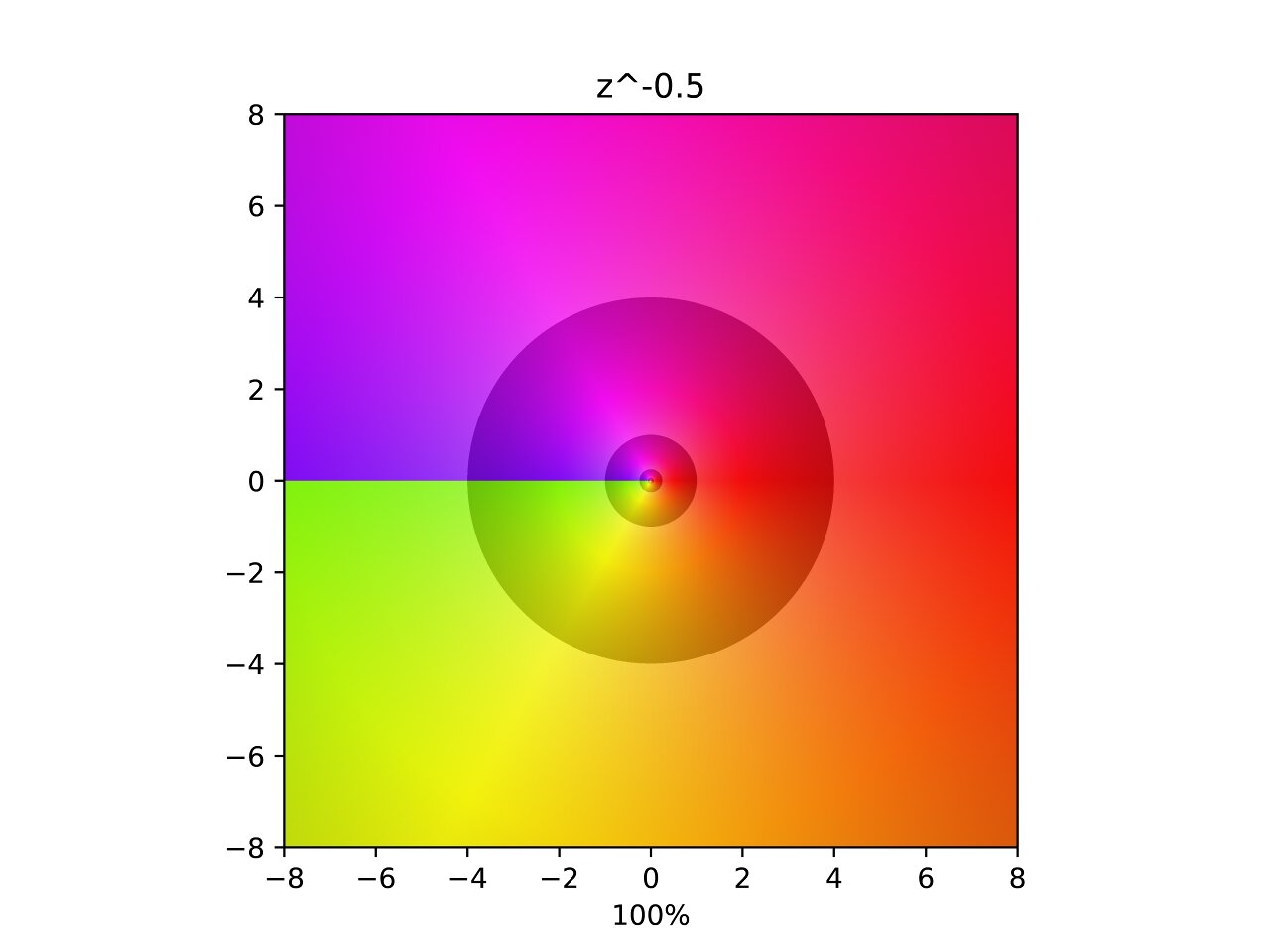
This one is similar to the last except that two poles are removed from the original at symmetric angles. This sheds some light on the previous function. I would guess that the previous interpolation also had moving poles, but they were hidden behind the branch cut.
Power of i
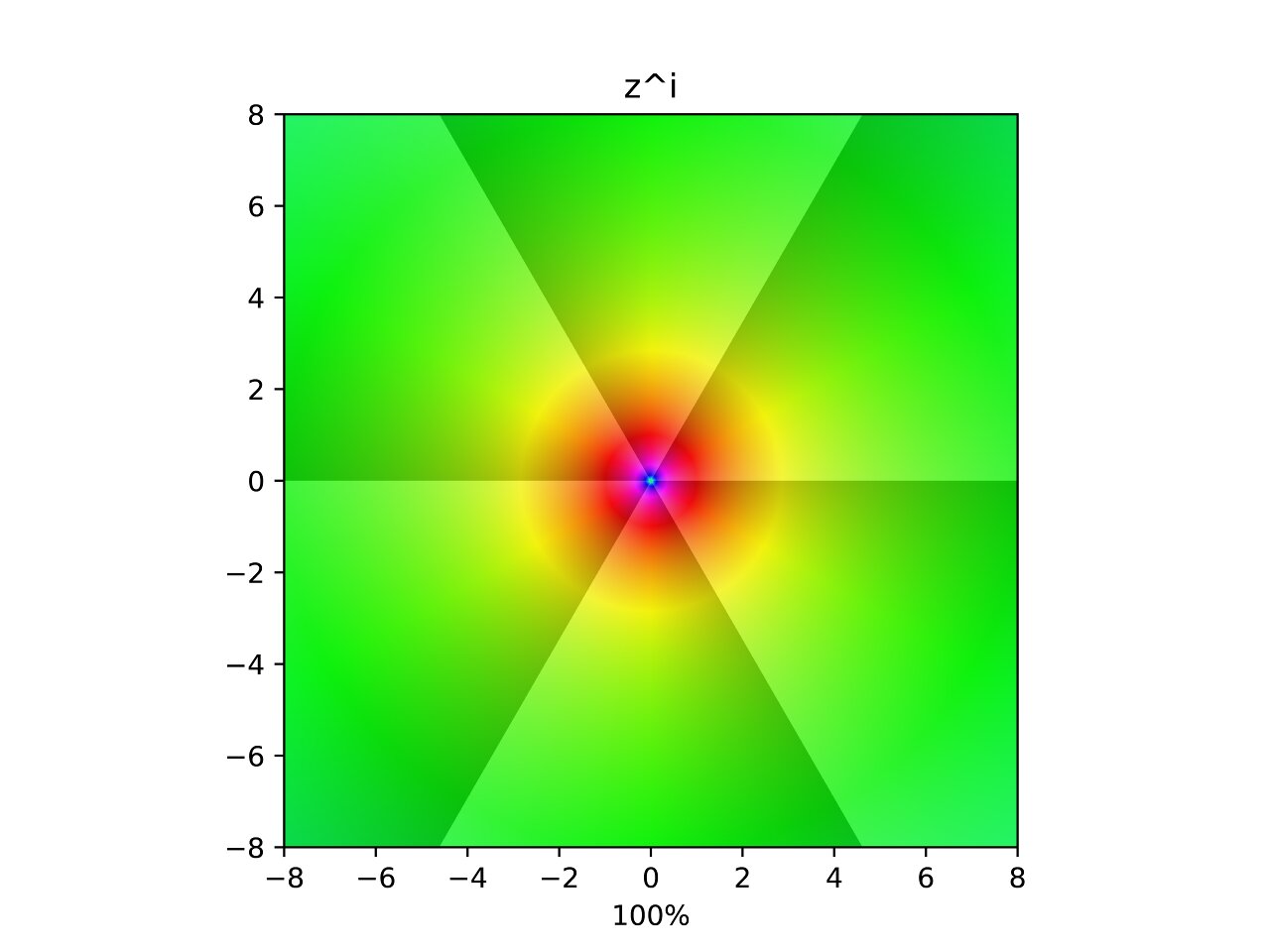
Now things are beginning to get funky. Taking the plane to the power of \(i\) seems to invert it in a different sense. The values now halve with angle, and are rotated counter-clockwise with magnitude. The interpolation shows two poles being removed in an asymmetric spiral fashion. I have slightly adjusted the contours to show powers of \(\mathrm{e}^{\frac{2\pi}{6}}\approx 2.85\) instead of \(2\), this causes the contours in the transformation to cleanly split the plane into \(6\) segments.
Power of -i
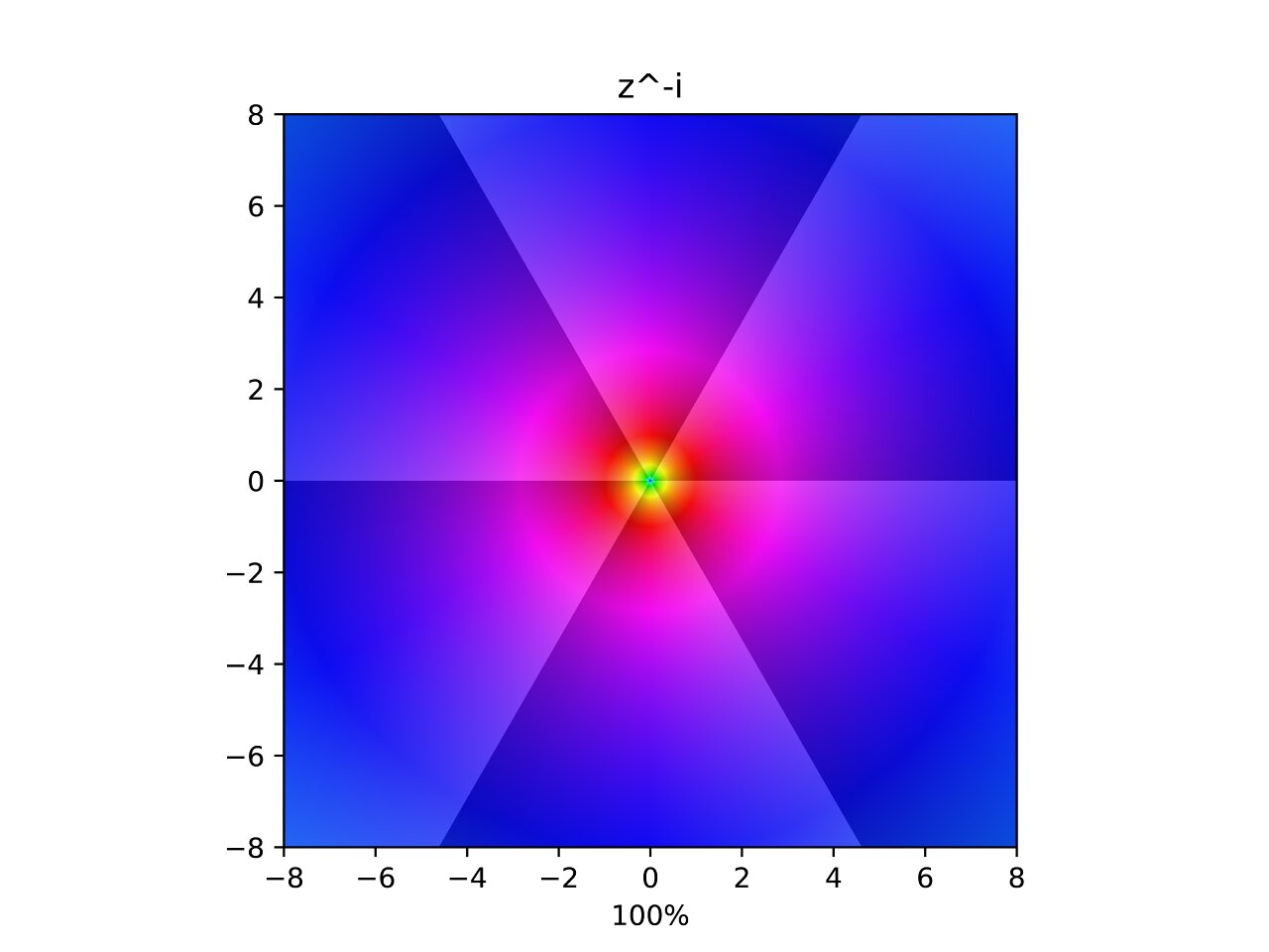
Similar to the last one but values are now doubled with angle, and are rotated clockwise with magnitude. I find it interesting that all the power interpolations involving merging or splitting poles in varying directions.
Sine
.jpg)
This is beautiful and one of my favourites. Poles merge from the top and bottom, only to immediately split again forming a colourful symmetric wave. Cosine is similar but shifted horizontally.
Hyperbolic Sine
.jpg)
Sine’s relationship to its hyperbolic counterpart becomes clear with these last two plots.
Arcsine
.jpg)
Doesn’t seem very interesting, but I’m curious to see what is going on beyond the branch cut.
Tangent
.jpg)
A sequence of alternating regular and inverse poles appear along the horizontal.
Sine of the Inverse
.jpg)
Recall how the limit of \(\sin(\frac{1}{x})\) is undefined as \(x\) approaches \(0\)? That is because sine begins oscillating wildly, not settling on any value. Now extend that concept to the complex values and you get this trippy singularity.
Tangent of the Inverse
.jpg)
I’m not even going to attempt to explain this nonsense.
Exponential
.jpg)
Poles pull in from right to left, flattening the contours into a clean horizontal sequence. The new magnitude is the exponential of the real component and the new angle is the imaginary component in radians.
Logarithm
.jpg)
Hard to see what’s going on here but this interpolation is unfolding into an infinite spiral beyond the branch cut. This means there are infinite solutions to any logarithm in the complex domain. The value that is returned is decided by where the branch cut is placed. The branch cut is usually placed such that the logarithm returns values with an angle greater than \(-\pi\) and less than or equal to \(\pi\).
Sigmoid
^-1.jpg)
The sigmoid is a function often used in neural networks because it restricts the output of reals between \(0\) and \(1\). Opposing poles appear out of thin air along the imaginary axis and pull back, leaving a sequence of vertical contours on the negative real side of the function in similar manner to \(\mathrm{e}^z\).
Softplus
.jpg)
Softplus is also found as an activation function of neural networks. Two poles seem to pull out from under the main branch cut to the right of the origin, which barely changes at all.
Gamma
.jpg)
The gamma function is a continuous version of the factorial. More specifically, \(\Gamma(n) = (n - 1)!\). This function is another favourite of mine, it looks quite exotic.
Expoid
.jpg)
This is a function I made up while playing around and ended up being interesting. I dub thee the expoid function. The black areas are where the calculations exceed the limits of floating point arithmetic on my computer, that area would be otherwise filled in with ever more compact fluctuations.
It seems as though up until the very last frame pillars of stability and instability form on the negative real side of the plot. Each pillar appears to approach a width of \(\pi\). This phenomena forms because when the imaginary component is a multiple of pi, the sign of the inner exponential becomes positive or negative. This causes the outer exponential to explode or vanish, both causing the same black artifact due to the how floating point numbers are stored. When the imaginary component is right between those multiples, the inner exponential becomes a pure imaginary number. The outer exponential then only rotates instead of changing magnitude, which is why those areas render properly.
Soft Exponential
The soft exponential is a rather rare activation function found in machine learning. It is a parameterized function \(f(a, z)\) where \(a\) is a parameter that interpolates the function between acting as the natural logarithm or the natural exponential. The important values of \(a\) are:
\[\begin{split} f(-1, z) &= \ln(z) \\ f(0, z) &= z \\ f(1, z) &= \mathrm{e}^z \\ \end{split}\]Riemann zeta function
.jpg)
.2.jpg)
Finally, the granddaddy of complex functions: The Riemann zeta function. Why is this function so important? Because it’s related to the distribution of primes, which is mysterious itself. If you can prove the Riemann hypothesis, you’ll have also proved a bunch of other results about the distribution of primes that rely on the hypothesis being true. You’ll also have won yourself one million dollars, but that’s not as important.
What is the hypothesis exactly? It’s that every nontrivial zero of the zeta function has a real part of \(\frac{1}{2}\). When I say trivial zeros, that means the poles on the negative real axis you can see in the images above. In the second image you can see the first two nontrivial zeros. These lie at about \((\frac{1}{2} + 14.1i)\) and \((\frac{1}{2} + 21.0i)\). There seems to be a pattern, but no one has proved it with absolute certainty yet.
Conclusion
Math is beautiful and visualizations can help foreign concepts become a little more intuitive. I hope this sparks someone’s interest in learning more about complex number systems. There are infinitely many, but they quickly become complicated so only the first few are often discussed.
What’s really interesting about them is you lose something each time you go to a higher algebra.
- Complex numbers lose ordering.
- Quaternions lose commutativity.
- Octonions lose associativity.
- Sedenions and higher lose alternativity and have nontrivial zero divisors
Check out Riemann surfaces for another powerful visualization tool that can also show what is happening beyond the branch cut.
Your domain coloring looks truly excellent! The font looks very much like matplotlib, do you have an example script?
Thanks, yeah I still have the scripts and they indeed use matplotlib, but they were never meant to see the light of day.
https://github.com/vankessel/sandbox/tree/master/graph
If I remember correctly
interp.pyandinterp2.pyare similar scripts used for these visuals.interp.pygenerated most of these interpolations.interp2.pyfor the interpolations that don’t bounce back and forth between identity and the mapping. You can ignoremain.pyHere’s a short summary I’ve given others who’ve asked about this code: